Compiler architecture
This overview assumes you have read the "Getting started" guide. The other pages in this section cover individual parts in detail.
Scaly is a compiler rather than a translator from expressions to C. Its
passes exploit the mathematical structure of a model, such as sparsity and
repeated stages, and they decide low-level properties of the generated code,
such as loops and memory layout. Like
Triton and
Warp, it compiles an embedded
domain-specific language (eDSL). Here the language is the Expr values written
inside a function decorated with @sc.function. Tracing the function captures
an intermediate representation (IR), a series of optimization passes transforms
it, and a final stage renders it as C code.
The diagram below summarizes this pipeline. The tools, libraries and compilers that influenced the design are described on a separate page.
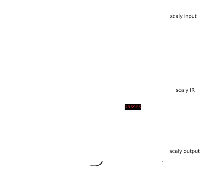
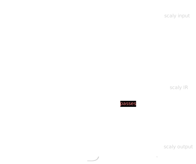
Tracing
The @sc.function decorator runs your Python body once, with symbolic inputs.
Each operation on an Expr builds a node of a graph instead of computing a
number. When the body returns, the graph it built is all that remains of it.
This is also why shapes are fixed: every shape is known when the graph is built.
The other way to compile an eDSL is source transformation, which reads the
function's Python source and translates its syntax, loops included. Scaly does
not do this. A Python for loop runs during tracing, so the graph contains it
unrolled, one copy of the body per iteration. The single-shooting rollout in
Getting started is
an example.
Calling a Function symbolically adds a single call node rather than copying
the callee's graph, and sc.vmap adds a single mapped-call node. These are how
a repeated calculation stays one node in the graph instead of many.
What an IR is
An intermediate representation, or IR, is a data structure that stores a computation in a form a compiler can analyze and transform. It is independent of the language the user wrote and of the code the compiler will emit. Python syntax is gone by the time the IR exists, and C syntax does not exist yet.
Scaly's IR is the graph that tracing builds, and its nodes are the Expr values
you already use. Each node is one operation. An Expr stores the operation tag
in op, its operands in args, its shape and data type in type, and
operation-specific data, such as the indices of a gather, in attrs. After
lowering, the nodes are ProgramNodes instead, with the same op, args and
attrs fields and a dtype. The next section explains why
there are two kinds of node.
Here is a small graph built by hand:
import scaly as sc

x = sc.sym("x", 3)
y = (x.sin() + x * x).sum()

y.op                        # ExprOp.SUM
y.type.shape                # ()
s = y.args[0]
s.op                        # ExprOp.ADD
[a.op for a in s.args]      # [ExprOp.SIN, ExprOp.MUL]
s.args[1].args[0] is x      # True
The output y is the root, and following args downward reaches every node
down to the input x. Both operands of x * x are the node x itself, so the
structure is a directed acyclic graph rather than a tree. Wrapping the same
computation in a Function and printing it with sc.render_expr_assembly lists
one node per line, operands before their users:
expr.func @f(%x: tensor<3xfloat64 diff>) -> (%y: tensor<float64 diff>) {
  %0 = expr.input {name="x"} : tensor<3xfloat64 diff>
  %1 = expr.sin(%0) : tensor<3xfloat64 diff>
  %2 = expr.mul(%0, %0) : tensor<3xfloat64 diff>
  %3 = expr.add(%1, %2) : tensor<3xfloat64 diff>
  %4 = expr.sum(%3) : tensor<float64 diff>
  expr.return %4
}
Assembly is only a textual form
"Assembly" here means the IR's textual form, not machine assembly language. The syntax is modelled on MLIR's textual format, but Scaly does not use MLIR and these listings are not valid MLIR. Influences says what Scaly took from it.
Scaly transforms the IR progressively through passes. Passes simplify it, differentiate it, lower it, optimize it and finally render it as C.
Why two dialects
A dialect is a set of operations with its own types and rules. Scaly's IR has two, one for mathematics and one for execution, and a program moves from the first to the second exactly once.
The expression dialect records what each value means. sc.sumsqr(x) is a
multiplication and a sum over whole arrays. Nothing is said about loops, memory
or evaluation order. This is the level where mathematics is easy. The derivative
of a sum is a rule of one line. x - x is visibly zero. A mapped call is
visibly the same stage function applied at every step of the horizon, so its
derivative can be one stage derivative applied at every step.
The program dialect records how to compute each value. Buffers, loops, loads,
stores and procedure calls are explicit. Lowering the function above gives a
store of zero into the output, a loop over x and an accumulating store in its
body, as printed by sc.render_program_assembly with some attributes trimmed:
prog.proc @f(%x: memref<3xfloat64>, %y: memref<1xfloat64>) {
  prog.store 0, %y[0] : float64
  prog.for %i_y = 0 to 3 step 1 {kind=reduce} {
    %v0 = prog.assign prog.load %x[%i_y] : float64 {declare=True}
    prog.store prog.add(prog.load %y[0], prog.add(prog.sin(%v0), prog.mul(%v0, %v0))), %y[0] : float64
  }
}
This is the level where code is easy to improve: merging two loops, expanding a small loop into scalar statements, reusing a temporary buffer once its value is dead.
Each level is hard to reach from the other. Recovering "this is a sum" from an accumulator loop means rediscovering what the user already said, and deciding where a temporary lives means nothing while the graph is still made of whole arrays. So Scaly does all the mathematical work first, in the expression dialect, and only then commits to loops and memory. Lowering is the one step between them, and nothing flows back up.
Properties of the IR
Nodes are values, defined once. An expression node is an immutable value with a fixed type,
and nothing can reassign it. The expression dialect is therefore in static single assignment
(SSA) form, which the listing shows directly: each %n appears on the left of exactly one line.
The program dialect is different where it has to be. Buffers are memory, and a store writes to memory, so statements inside a block run in order and a later store can overwrite an earlier one. The nodes themselves are still immutable, and the scalar arithmetic inside a statement is still a graph of values.
Equal nodes are the same node. Both dialects intern their nodes. Building a node whose
operation, operands, type and attributes match an existing node returns the existing node. So
writing x.sin() twice gives one sine, and x.sin() is x.sin() is true. This common
subexpression elimination (CSE) happens as the graph is built, with no pass to run, and it holds
across all the graphs alive in a process. It is why the gradient of x * x computes x times the
seed once and adds that node to itself. The intern tables hold weak references, so unused nodes
are still garbage-collected. An explicit sc.cse pass remains for the cases interning cannot see.
Every node has a static type. An expression node's TensorType holds a fixed shape, a data
type and a differentiability flag. Program buffers have fixed shapes too. Nothing in the generated
code allocates memory or checks a shape at run time, because no shape can change after tracing.
Each dialect has a verifier. A table of rules states which operands, types and attributes each
operation accepts. Construction checks common mistakes as nodes are built, and sc.verify_expr and
verify_program check a whole graph. Lowering verifies its result, so a malformed program fails
before any C exists.
Everything is a pass
A pass reads a graph and either returns a new graph or reports a fact about it. Scaly's stages are all passes of this kind, sorted by what they consume and produce:
| Pass | From | To |
|---|---|---|
| Simplification and CSE | Expression graph | Expression graph |
| Sparsity analysis | Expression graph | A sparsity pattern |
| Differentiation | Expression graph | Expression graph |
| Lowering | Expression graph | Program |
| Program optimization | Program | Program |
| Rendering | Program | C source |
A pass never modifies a graph. It traverses the graph and builds a new one, and the old graph stays valid. Scaly relies on this when it simplifies a private copy of a graph before lowering while keeping the original for differentiation and inspection. Interning keeps this cheap. A part of the graph that a pass leaves unchanged comes back as the very same nodes.
A sparse Jacobian shows how passes compose. Asking for one runs, in order:
- Sparsity analysis. Walks the expression graph and tracks which input elements each output element can depend on. No numbers and no derivatives are involved, and the result is the structural pattern of the Jacobian.
- Coloring. Groups the pattern's columns so that each group can share one forward-mode direction. This works on the pattern alone.
- Differentiation. Applies the chain rule node by node for each direction, building new
expression nodes, then gathers the compressed results into an array of nonzero values. The
result is a new
Functionwhose output carries the pattern.
Nothing in that sequence knows the derivative will become C. The new Function is an expression
graph like any other. You can differentiate it again to get a second derivative, call it inside a
larger graph, or evaluate it. Evaluating it sends it down the same path as the original:
simplification, lowering, program optimization and rendering. A numerical call then compiles the C
and loads it.
This is the model to keep in mind when reading the rest of Scaly. A new feature is usually a new pass or a new rule inside an existing pass. The question to ask is which dialect has the information the feature needs. Mathematical facts are in the expression dialect, and memory and loop facts are in the program dialect.
Where each part lives
| Part | Location |
|---|---|
| Both dialects, their verifiers, the rewrite driver | src/scaly/ir/ |
Tracing and the Function boundary |
src/scaly/function/ |
| Differentiation and sparsity analysis | src/scaly/ad/ |
| Expression rewrites, lowering, program optimization | src/scaly/passes/ |
| Rendering, compiling and loading | src/scaly/codegen/ |
The codebase has the module-level map.