Modeling Workflow

A continuous-time optimal control problem is transcribed into a finite-dimensional mathematical program, which is then passed to a numerical solver. The resulting solver object can be called repeatedly and returns the optimized trajectories to the application.

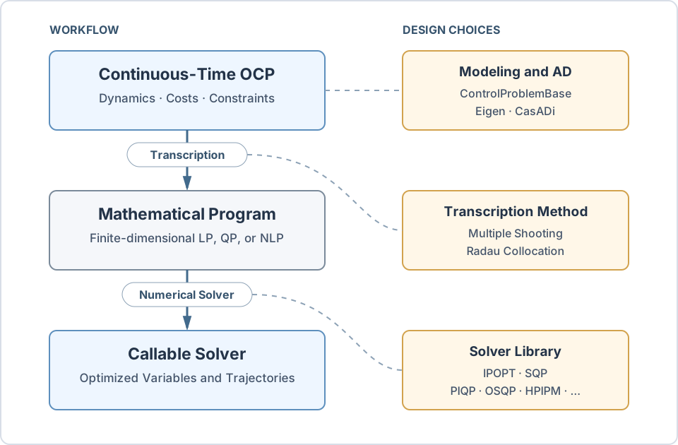
The stages are deliberately independent. A model can be paired with different transcription methods, and the resulting nonlinear program can be paired with different solvers without rewriting the model equations.

Memory ownership: Each layer owns its memory and keeps the layer below it alive: the transcription owns the OCP, the Problem owns the transcription, and the solver owns the Problem.

1. Formulate the Continuous-Time OCP

The user defines the dynamics, running and terminal costs, bounds, and optional path constraints through laopt_tools::ControlProblemBase. These functions remain close to their mathematical form and operate on fixed-size Eigen vectors.

The modeling layer also determines how derivatives are obtained. Eigen-based automatic differentiation (AD) is the default, while CasADi can be selected for supported derivative configurations.

using Ocp = InvertedPendulum;
auto ocp = std::make_shared<Ocp>();

At this stage, the model is continuous in time. It does not yet contain shooting nodes, collocation points, or solver-specific data structures.

2. Choose a Transcription

A transcription replaces the continuous trajectories with a finite set of decision variables and adds constraints that enforce the dynamics. laOPT currently provides multiple shooting and Radau collocation.

// Template parameters: OCP type, number of shooting intervals.
using Transcription = laopt_tools::MultipleShooting<Ocp, 40>;
auto transcription = std::make_shared<Transcription>(ocp);

The transcription controls the discretization and sparsity structure. Changing it does not require changing the OCP class:

// Template parameters: OCP type, number of mesh segments,
// and polynomial degree in each segment.
using Transcription = laopt_tools::RadauCollocation<Ocp, 10, 3>;

3. Construct the Mathematical Program

laopt::Problem turns the transcribed model into the solver-facing nonlinear program. During construction, laOPT discovers derivative sparsity and records the evaluation tape used for repeated numerical evaluations.

using Problem = laopt::Problem<Transcription>;
auto problem = std::make_shared<Problem>(transcription);

Applications that are not optimal-control problems can enter the workflow directly at this layer by defining a general NLP model. See Modeling Nonlinear Programs.

4. Select a Numerical Solver

The same Problem can be passed to an interior-point solver or the native laOPT SQP solver. SQP additionally requires a QP backend for its subproblems.

using QPSolver = laopt::PIQPSolver<double>;
using Solver = laopt::SQPSolver<Problem, QPSolver>;

Solver solver(problem);
solver.solve();

For an interior-point method, only the solver type changes:

using Solver = laopt::IpoptSolver<Problem>;

5. Read the Optimized Trajectories

The transcription owns the OCP-specific trajectory representation. After the solver updates the decision variables, read the solution through the transcription:

solver.solve();

Transcription::TimeTrajectory  T_opt = transcription->get_T_opt();  // 41 time nodes
Transcription::StateTrajectory X_opt = transcription->get_X_opt();  // NX × 41 states
Transcription::InputTrajectory U_opt = transcription->get_U_opt();  // NU × 40 inputs

std::cout << "final time: " << T_opt(T_opt.size() - 1) << '\n';
std::cout << "final state: " << X_opt.rightCols(1).transpose() << '\n';

For 40-segment MultipleShooting<Ocp, 40>, the state trajectory has 41 nodes and the input trajectory has one value per segment.

The getters return fixed-size vector/matrix types that the application can store or process independently. Instead of using the fixed types (e.g., Transcription::StateTrajectory), one can also use dynamic-size types (e.g., Eigen::MatrixXd) for storing and manipulating the results. The type can also be inferred using auto:

Transcription::StateTrajectory X_opt_1 = transcription->get_X_opt();
               Eigen::MatrixXd X_opt_2 = transcription->get_X_opt();
                          auto X_opt_3 = transcription->get_X_opt();

Design Choices at a Glance

Workflow Stage	Primary Choice	laOPT Components
OCP formulation	Model and derivative backend	ControlProblemBase, Eigen AD, CasADi
Transcription	Discretization method and resolution	MultipleShooting, RadauCollocation
Mathematical program	General NLP representation	Problem<Transcription>
Numerical solution	NLP method (and QP backend)	IpoptSolver, SQPSolver, (PIQPSolver, and other QP interfaces)

This separation is the central modeling principle in laOPT: formulate the control problem once, then choose the transcription and solver combination appropriate for the application.