First Optimal Control Problem (OCP)
This example uses laOPT’s high-level optimal-control interface to swing an inverted pendulum from the downward position to the upright equilibrium. The nonlinear OCP is
\[\begin{aligned} \min_{\theta,\omega,u}\quad & \int_0^{1.5} \left(10 \cdot \theta^2 + u^2\right)\,dt + 100 \cdot \theta^2 \\ \text{s.t.}\quad & \begin{pmatrix} \dot{\theta} \\ \dot{\omega} \end{pmatrix} = \begin{pmatrix} \omega \\ \frac{mgl\sin\theta-b\omega+u}{ml^2} \end{pmatrix}, \\ & \begin{pmatrix} \theta(0) \\ \omega(0) \end{pmatrix} = \begin{pmatrix} \pi \\ 0 \end{pmatrix}, \\ & -3 \leq u \leq 3. \end{aligned}\]The target is \(\theta=0\). Multiple shooting turns the continuous-time OCP into a nonlinear program, and laOPT’s SQP solver solves its quadratic subproblems with PIQP.
Define the OCP
Derive from ControlProblemBase and implement the dynamics, running cost, and terminal cost. The base-class template arguments specify two states and one input.
#include <laopt/laopt.hpp>
#include <laopt/tools/control_problem_base.hpp>

class InvertedPendulum : public laopt_tools::ControlProblemBase<double, 2, 1>
{
public:
    // Running cost: keep the angle near zero while limiting torque.
    template <typename X, typename U, typename P,
              typename T0, typename TF, typename Tau,
              typename Scalar = typename X::Scalar>
    Scalar lagrange_term_impl(const Eigen::MatrixBase<X>& x, const Eigen::MatrixBase<U>& u,
                              const Eigen::MatrixBase<P>& p,
                              const Eigen::MatrixBase<T0>& t0, const Eigen::MatrixBase<TF>& tf,
                              const Tau& tau)
    {
        unused(p, t0, tf, tau); // Just to surpress annoying compiler warnings
        return 10.0 * x(0) * x(0) + u(0) * u(0);
    }

    // Terminal cost: strongly penalize the final angle error.
    template <typename XF, typename P, typename T0, typename TF,
              typename Scalar = typename XF::Scalar>
    Scalar mayer_term_impl(const Eigen::MatrixBase<XF>& xf, const Eigen::MatrixBase<P>& p,
                           const Eigen::MatrixBase<T0>& t0, const Eigen::MatrixBase<TF>& tf)
    {
        unused(p, t0, tf); // Just to surpress annoying compiler warnings
        return 100.0 * xf(0) * xf(0);
    }

    // Nonlinear pendulum dynamics.
    template <typename X, typename U, typename P,
              typename T0, typename TF, typename Tau,
              typename Scalar = typename X::Scalar>
    state_t<Scalar> dynamics_impl(const Eigen::MatrixBase<X>& x, const Eigen::MatrixBase<U>& u,
                                  const Eigen::MatrixBase<P>& p,
                                  const Eigen::MatrixBase<T0>& t0, const Eigen::MatrixBase<TF>& tf,
                                  const Tau& tau)
    {
        unused(p, t0, tf, tau); // Just to surpress annoying compiler warnings

        const double g = 9.81;
        const double l = 0.5;
        const double m = 0.15;
        const double b = 0.1;

        const Scalar theta = x(0);
        const Scalar omega = x(1);
        const Scalar torque = u(0);

        state_t<Scalar> x_dot;
        x_dot << omega,
                 (m * g * l * sin(theta) - b * omega + torque) / (m * l * l);
        return x_dot;
    }
};
Transcribe and Solve
The solve code stays independent of the model equations. It sets the horizon and bounds, selects a transcription and QP backend, and recovers the optimized trajectory.
#include <iostream>
#include <memory>

#include <laopt/solvers/piqp_interface.hpp>
#include <laopt/solvers/sqp_solver.hpp>
#include <laopt/tools/multiple_shooting.hpp>

int main()
{
    using Ocp = InvertedPendulum;

    // Discretize the OCP with 40 multiple-shooting intervals.
    using Transcription = laopt_tools::MultipleShooting<Ocp, 40>;
    using Problem = laopt::Problem<Transcription>;
    using QPSolver = laopt::PIQPSolver<double>;

    auto ocp = std::make_shared<Ocp>();
    auto transcription = std::make_shared<Transcription>(ocp);
    auto problem = std::make_shared<Problem>(transcription);

    // Start downward and optimize over a fixed 1.5-second horizon.
    ocp->set_x0(Ocp::State{3.14159, 0.0});
    ocp->set_tf(1.5);
    ocp->u_lb << -3.0;
    ocp->u_ub << 3.0;

    // Use PIQP for the SQP subproblems and print iteration progress.
    laopt::SQPSolver<Problem, QPSolver> solver(problem);
    solver.settings().verbose = true;
    solver.solve();

    // Recover the optimized state trajectory.
    const Eigen::MatrixXd X = transcription->get_X_opt();
    std::cout << "terminal state: " << X.rightCols(1).transpose() << '\n';
}
The verbose solver output shows the progress of each SQP iteration:
----------------------------------------------------------
                        laOPT SQP
    (c) Roland Schwan, Johannes Waibel, Colin N. Jones
   Ecole Polytechnique Federale de Lausanne (EPFL) 2026
----------------------------------------------------------
variables n = 122
constraints m = 80
lagrangian hessian nnz = 81
constraints jacobian nnz = 320
globalization strategy: LINE_SEARCH_FILTER
iter    objective     primal_inf    comp_inf      stat_inf      alpha       qp_iter   elastic
   0    0.00000e+00   3.14159e+00   0.00000e+00   0.00000e+00   0.000e+00         0   0.00000
   1    3.00641e+00   2.06403e+00   1.52968e-01   4.74015e-01   3.430e-01         6   0.00000
   2    6.55798e+00   1.35607e+00   3.07628e-01   9.80883e-01   3.430e-01         6   0.00000
   3    1.50121e+01   4.76584e-01   4.14062e-01   5.77677e-01   1.000e+00         9   0.00000
   4    1.38895e+01   1.37858e-02   7.32745e-04   1.44423e-02   1.000e+00         7   0.00000
   5    1.38865e+01   4.62268e-08   1.19148e-09   1.59571e-05   1.000e+00         7   0.00000
status: SOLVED
sqp iterations: 5
qp iterations: 35
terminal state: 8.56714e-08  -0.0020322
Optimized Trajectory
The optimized torque swings the pendulum upright and settles both the angle and angular velocity near zero.
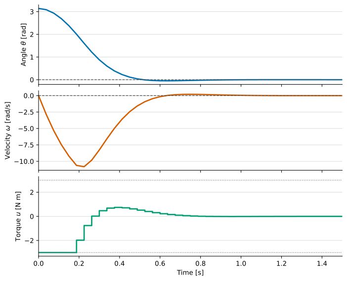
Use get_T_opt(), get_X_opt(), and get_U_opt() to retrieve the complete optimized trajectories. The Optimal Control section describes other costs, constraints, and transcription methods.